Data analysis? dplyr is your ally

One of the most used tools for data analysis is R, this software has native functions that can help us when cleaning or wanting to extract some information from our datasets. However, many of these operations can be tedious to write, to demonstrate this we will use a dataset from Kaggle on human population. After downloading the .csv file we will proceed to load it into RStudio.

library(readr)
popData <- read_csv(file = "./world_pop/world_population.csv")

Imagine that we want the ranking and the abbreviation for Chile, in the case of native R code, this would be done like this:

popData[which(popData$Country == "Chile"), names(popData) %in% c("Rank", "CCA3")]

While with dplyr we would do this:

popData %>%
filter(Country=="Chile")%>%
select(Rank,CCA3)

In the dplyr package there are several functions that will help us manipulate our dataframes, which we can divide into functions to summarize information (summarise, count), to group cases (group_by, rowwise, ungroup), Manipulate cases (filter, distinct, slice, slice_sample, slice_min, slice_head, arrange, add_row), Manipulate variables (pull, select, relocate, across, c_across, mutate, transmute, rename). Let’s review some of these functions.

The first element that dplyr brings us and I didn’t mention before is the pipe (%>%) we can concatenate the results of a function and apply another one directly to it.

head(popData) # Without pipe use

popData %>%
  head() # With pipe use

Select()

Now yes, let’s go to the Dplyr functions, we will start with select(), this allows us to select columns from our data frame indicating its name. Let’s see, let’s select the continents from our data set.

popData %>%
  select(Continent)

This generates a dataframe of a single column with the continents.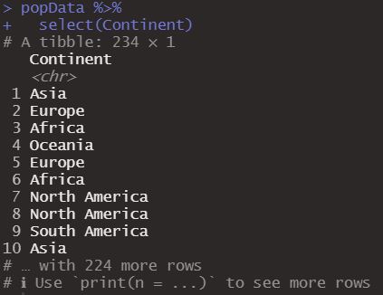

We can also select more than one column and rename the Growth Rate column.

popData %>%
  select(Country, Continent, Growth_Rate = 'Growth Rate')

Now we have a data frame with three columns.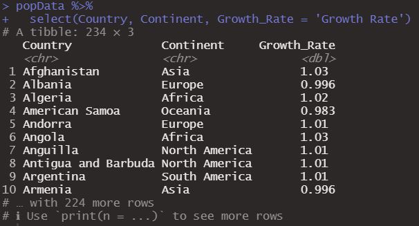

We can also rename a column by calling the rename function of dplyr, like this:

popData %>%
  select(Country, Continent, 'Growth Rate') %>%
  rename(Growth_Rate = 'Growth Rate')

As you see there is not only one way to carry out these tasks and the use of the pipe %>% makes it much easier to use one function after another.

Another thing we can do with select is to use helper functions, in this case we use ends_with to select all columns that end with “Population”:

popData %>%
  select(ends_with("Population"))

Thus checking the following dataframe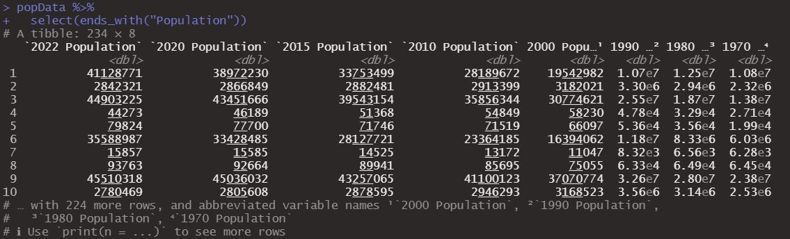

Relocate()

The second function that we will briefly see is relocate, which as its name says allows us to change the order of a column in the data frame. We can for example indicate that the Country column remains as the last one using the .after parameter.

popData %>%
  select(Country, Continent, 'Growth Rate') %>%
  rename(Growth_Rate = 'Growth Rate') %>%
  relocate(Country, .after = last_col())

Obtaining the following dataframe.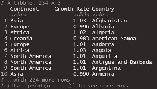

We could leave it before the last column changing after for before.

popData %>%
  select(Country, Continent, 'Growth Rate') %>%
  rename(Growth_Rate = 'Growth Rate') %>%
  relocate(Country, .before = last_col())

Obtaining the following dataframe.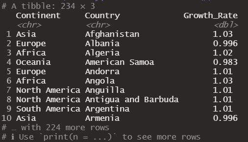

We can even reference another column to position the target column, let’s put Country after Continent.

popData %>%
  select(Country, Continent, 'Growth Rate') %>%
  rename(Growth_Rate = 'Growth Rate') %>%
  relocate(Country, .after = Continent)

Obtaining the same dataframe that we obtained in the previous example.

Mutate()

Continuing with column operations we have the mutate function, which allows us to create a new column. For example a new column could be a projection of the population in 2023, by multiplying the growth rate by the population of each country in 2022. We could also obtain a column with the difference in population number between 2022 and 2020 or even calculate the logarithm of the 2022 population. We can do this separately or even in a single line of code.

popData %>%
  mutate(Proy_2023 = `2022 Population` * `Growth Rate`) %>%
  mutate(Dif_betw_22_20 = `2022 Population` - `2020 Population`) %>%
  mutate(log_2022 = log(`2022 Population`)) %>%
  select(Proy_2023, Dif_betw_22_20, log_2022) #Multiple lines case

popData %>%
  mutate(Proy_2023 = `2022 Population` * `Growth Rate`,
         Dif_betw_22_20 = `2022 Population` - `2020 Population`,
         log_2022 = log(`2022 Population`))%>%
  select(Proy_2023, Dif_betw_22_20, log_2022) #Single line case

Obtaining in both cases the following dataframe.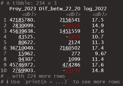

If you notice, the name of the column goes before the operation that defines it, we also combine what was obtained through mutate with the select() function to observe the new columns created.

Functions that manipulate rows

Now we will review the functions that manipulate cases or rows. Perhaps one of the most important is the filter function.

Filter()

This function as its name indicates allows us to filter our data set to obtain only the observations we desire, for example we could obtain information only from Chile, by filtering Country and searching for Chile.

popData %>%
  filter(Country == "Chile")

We would obtain the following dataframe.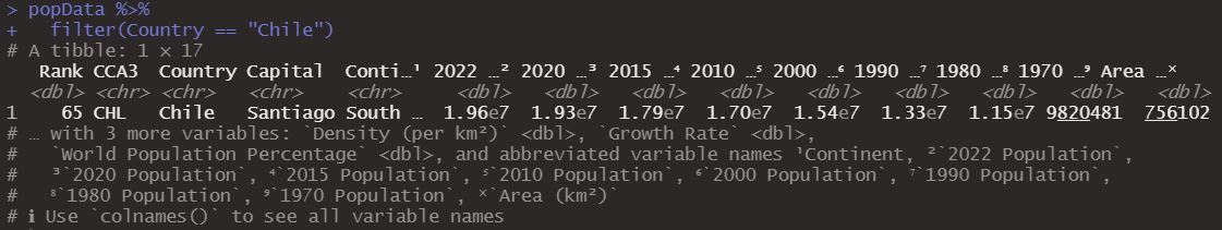

Before continuing it is important to mention that this function goes hand in hand with logical or boolean operators, which you can see over here.

We can filter using these operators and even combine them to obtain more precise filters. First we will filter by ranking, choosing those that are under rank 100 and are also countries from South America. We can do that same thing by using the logical operator AND, represented by this “&” character.

popData %>%
  filter(Rank < 100, Continent == "South America")

popData %>%
  filter(Rank < 100 & Continent == "South America")

Obtaining the following dataframe.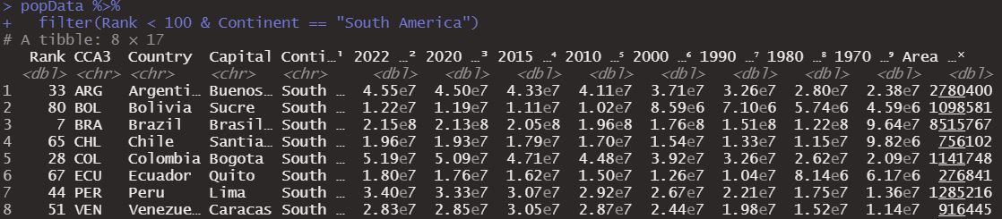

We might want those countries that are under rank 100, but that are not from South America, for that we would use the NOT operator, represented by !=.

popData %>%
  filter(Rank < 100 & Continent != "South America")

Obtaining the following dataframe.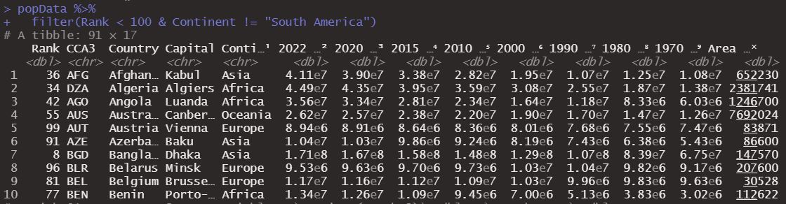

We could even filter to obtain again the countries under rank 100 or those that are from South America with the OR operator.

popData %>%
  filter(Rank < 100 | Continent == "South America")

Which gives us a dataframe similar to the previous one but that also contains all the countries of South America.

Arrange()

The second and last function of this category that we will review is arrange, which allows us to order the rows with respect to a value. For example let’s order these data based on the population in 2022.

popData %>%
  arrange(`2022 Population`)

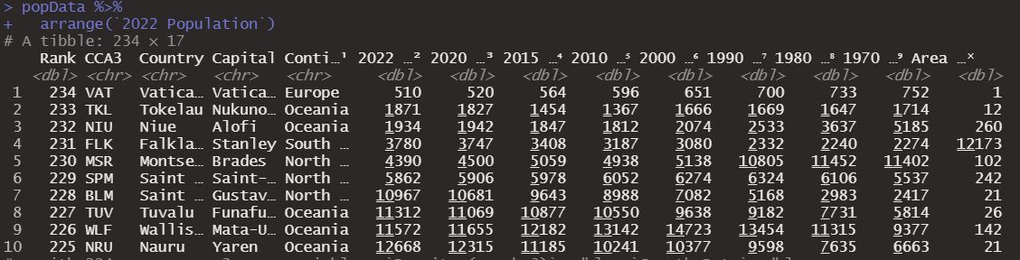
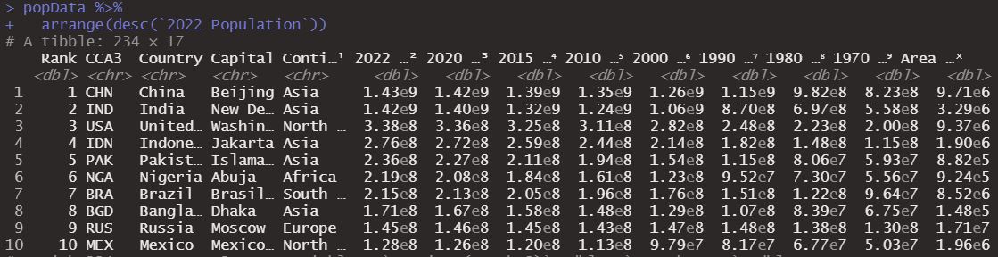
As we see it orders it from lowest to highest, we can change this to descending form using the desc function.

popData %>%
  arrange(desc(`2022 Population`))

And so we could order this data frame based on any variable, even those that we can create with mutate, let’s calculate again the difference between the population of 2022 and 2020 and order in relation to that calculation.

popData %>%
  mutate(dif_2020_2022 = `2022 Population`- `2020 Population`)%>%
  arrange(desc(dif_2020_2022))

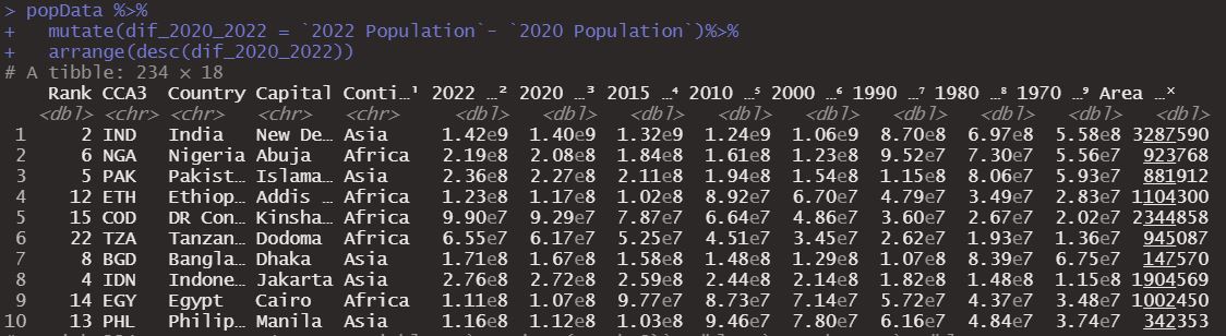
As we see India is now in first place followed by Nigeria and China is no longer in the top 10 places.

Functions to organize information

Finally we will review together a function to group group_by and on the other hand two functions to summarize information, count and summarise.

Group_by() and Summarise()

Group_by for its part allows us to group rows with respect to the values of a particular column, for example let’s group this data set based on the continents.

popData %>%
  group_by(Continent)

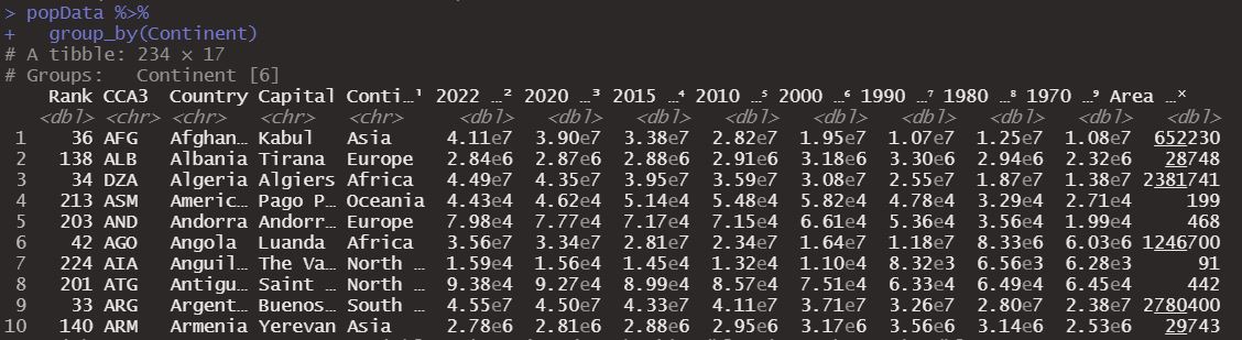
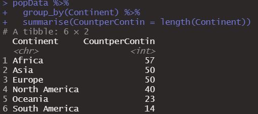
In principle we don’t see much change, but if we couple this function with summarise, which allows us to summarize information and create a column that tells us the total elements of each group created, we see how group_by can be a great function to help us summarize information, since it changes how the data set interacts with other dplyr functions.

popData %>%
  group_by(Continent) %>%
  summarise(CountperContin = length(Continent))

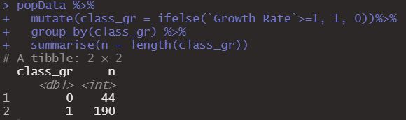
Another thing we can do is create a new variable with mutate and then group around that variable and obtain some summary of the information. Here we will classify the countries giving them a 1 when their growth rate is greater than or equal to 1 and a 0 when it is less than 1, then we will group by this variable and count how many countries there are in each class.

popData %>%
  mutate(class_gr = ifelse(`Growth Rate`>=1, 1, 0))%>%
  group_by(class_gr) %>%
  summarise(n = length(class_gr))

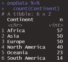
Count()

Finally the first exercise we performed in this section, we could have done it with count() in this way, much more direct, count serves us to count the cases of a variable or column of interest.

popData %>%
  count(Continent)

Even, although not very used, we can evaluate some condition inside count, for example let’s evaluate the condition of countries where the 2022 population is greater than 100000.

popData %>%
  count(`2022 Population` > 100000)

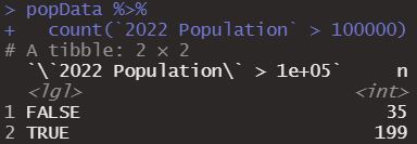
We see how it gives us a result both for when it is true and for when this condition is false.

With this we have reviewed some of the main functions of dplyr which would allow you to continue exploring this incredible package. It is possible to do much more, but without a doubt these functions will help you take your first steps.